
One of the first known applications of geometrical methods to an astronomical distance was from ancient Greece. Astronomers there noticed that the shadow of Earth on the Moon during a lunar eclipse was not a straight line, but a curved arc. Using the amount of curvature of the arc, they could deduce the size of Earth’s circular shadow, which could be directly compared to the apparent size of the Moon itself. In this way, they were able to deduce the relative sizes of Earth and its moon.

Earth’s size had been determined by the Greek scholar Eratosthenes (276–194 BCE), who used the geometry of circles and the lengths of shadows cast by vertical sticks to deduce Earth’s circumference (Figure 6.2). With the results of Eratosthenes in hand, it was possible to assign an absolute size to the Moon. Then, a mathematical estimate known as the small-angle approximation allowed its distance from Earth to be determined. So, more than 2,000 ago, Greek scholars knew that the Moon was about a quarter million miles from Earth, though they did not express the distance in miles, of course.

The small-angle approximation, also known as the small-angle formula, can be used to determine the distances to faraway objects.
The distance \(d\) to an object, is the ratio of its size, \(S\), and \(\theta\) (Greek letter “theta”), the angle in radians that the object spans from the location of a viewer (Figure 6.3). For the derivation of this formula, see Going Further 6.1: Derivation of the Small-Angle Approximation.
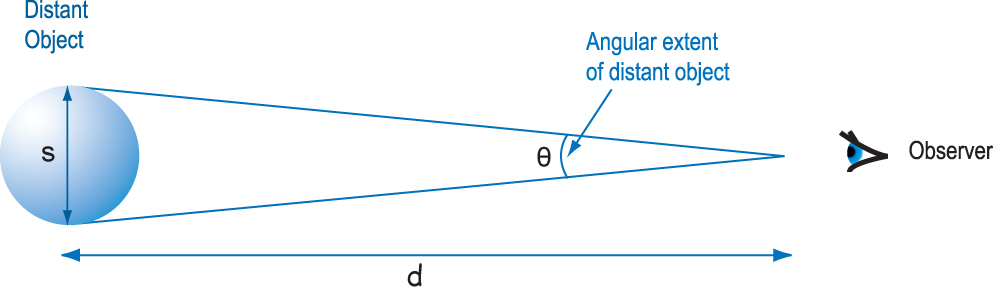
Mathematically, angular diameter, linear size, and distance can be combined in an extremely useful and simple equation called the small-angle approximation. As seen in Figure 6.3, the angular diameter, \(θ\), depends on the distance to the object, \(d\), and its actual linear size, \(S\), according to:
For very small values of \(θ\) measured in radians, \(\tan(θ) = θ\). Using this approximation, we can simplify the equation relating distance and linear size to:
In this small-angle approximation, if any two of the quantities are known, the third can be calculated. In astronomy, the angular diameter is usually measured directly, and the equation is used to calculate the distance to or physical size of the object. Since distances to astronomical objects are usually much larger than their linear sizes, this approximation is of great use in all branches and at all levels of astronomy!
The table below shows the relationship between the angle (in degrees and radians) and the tangent of the angle. Also shown is the difference between the angle in radians and the tangent of the angle. The close correspondence between these two quantities is the basis of the small-angle approximation.
| Angle (degrees) | Angle (radians) | Tangent (angle) | Difference | % Difference |
|---|---|---|---|---|
| 0.5 | 0.0087 | 0.0087 | 0.0000 | 0.0025 |
| 1.0 | 0.0175 | 0.0175 | 0.0000 | 0.0102 |
| 2.0 | 0.0349 | 0.0349 | 0.0000 | 0.0406 |
| 4.0 | 0.0698 | 0.0698 | 0.0000 | 0.1628 |
| 8.0 | 0.1396 | 0.1405 | 0.0009 | 0.6550 |
| 15.0 | 0.2618 | 0.2679 | 0.0066 | 2.349 |
| 20.0 | 0.3491 | 0.3640 | 0.0149 | 4.270 |
| 25.0 | 0.4363 | 0.4663 | 0.0300 | 6.870 |
| 30.0 | 0.5236 | 0.5774 | 0.0538 | 10.27 |
Based on looking at the table, when do you think the approximation breaks down?
The first distance measurement technique devised for distances outside of the Solar System involves a phenomenon that you see every day, though you may not have noticed it or realized how you could use it to measure distance. Parallax is the apparent shift in position of a foreground object relative to the background. This is how we perceive depth using the small differences in perspective as seen from our two eyes. We typically learn to estimate distances without having to think about it using this technique when we are very young. Astronomical parallax is a more formalized (mathematical) version of our binocular vision. To familiarize yourself with this fundamental distance measurement technique in astronomy, and to connect that measurement technique to everyday things, you should complete the following activity on parallax.
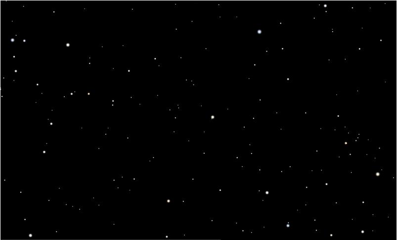
I n this activity you will use Figure A.6.1 as a backdrop simulating distant stars as we explore what happens when you view an object from two different perspectives.

When you observe relatively nearby stars against a backdrop of distant stars, the nearby stars will shift as Earth orbits around the Sun. Figure 6.5 illustrates this type of parallax. The drawing in the right-hand side of the figure shows the geometry of the setup as you look at a relatively close object against a distant background. These might be distant stars in the astronomical context, but the same principle applies to terrestrial viewing as well.
Now bring your attention to Figure 6.5. There are two simulated star fields, labeled 1 and 2. These correspond to viewing the same part of the sky from Earth, with viewing sessions separated by six months. At the left of the figure, View 1 and View 2 illustrate how the setup translates into what you would actually see from the two perspectives. Notice that the two parts of the figure illustrate the important point that the shift in position relative to the background stars represents a change in the angle that our line of site makes with the object relative to some reference line. Thus, parallax is an angle.

In Figure 6.6 we de-clutter the diagram to concentrate on the geometry. Consider the triangle shown in the figure. We can choose to do our measurements so that one of the angles of the triangle is a right angle (90°). The angle a is the parallax angle, which we can measure by the apparent shift of the nearby star. Note that it is half the apparent angular shift that the star makes between the two measurements, 1 and 2. This is because we have drawn the triangle to have a right angle, a choice made for convenience, not necessity.
An important point to notice about the triangle is that if you make the distance d bigger (keeping the baseline B the same), the parallax angle a gets smaller, while if you make B bigger (keeping d the same), the parallax angle a gets bigger. This matches with the qualitative relationship you found in the activity when you viewed your thumb at different distances from your face.

Next, we need to calculate the distance quantitatively. We can do this using trigonometry to relate angles to ratios of distances and using the definition of the tangent to write the following relation.
If we know \(B\) and measure \(a\), we can calculate the distance \(d\).
This technique for measuring distances is commonly used in surveying for roads or buildings.
In astronomy, the parallax angle is always very tiny because the distances to objects are so huge. The baseline B is the radius of Earth’s orbit around the Sun, and even with such a “large” baseline, the largest parallax angles are still less than 1/4,000th of a degree! To describe such small angles the degree is split into small divisions of arcminutes (1/60th of a degree, symbolized by ‘ or arcmin) and arcseconds (1/60th of an arcminute, symbolized by “ or arcsec). The parallax angles for even the nearest stars are less than 1 arcsec. Therefore, the small-angle approximation holds in these cases, and we can rewrite the equation for parallax as:
This formula is consistent with what we found in the activity: the farther the distance, the smaller the parallax shift. The bigger the baseline, the bigger the parallax shift. But we emphasize, this version of the formula only works when the angle is measured in radians, not degrees, arcseconds, or arcminutes. So, sometimes, we must use the fact that there are pi (\(\pi\)) radians in 180 degrees to convert angles between degrees and radians if we want to use the small-angle formula. And, to re-emphasize, the angle must be small, a condition always satisfied when measuring astronomical parallax to a star.
You have learned about two basic ways to describe the size of an angle. The first uses degrees, arcminutes, and arcseconds. The second uses radians. In the next activity you will learn how to convert between these units. Then you will practice using the parallax formula.
1. Convert 30 degrees to arcseconds.
2. Convert 30 degrees to radians.
Sometimes, astronomers use a distance unit called a parsec to describe distances. Parsec is short for parallax-second and is abbreviated pc. When the baseline B is the distance between Earth and the Sun (1 AU) and the parallax angle a is measured in arcseconds (arcsec for short), then the distance d has units of parsecs. In this case, our formula for distance becomes:
\(d\) (in pc) \(=1/a\) (in arcsec)
For example, this means that if a star has a parallax angle of 1 arcsec, it is at a distance of 1 parsec; if a star has a parallax angle of 1/2 arcsec, it is at a distance of 2 parsecs. We emphasize: this version of the formula only works when the angle is measured in arcsec and the distance is measured in parsecs. Parsecs are a convenient way to keep track of the relative distances of stars. If absolute distances are needed, it is simple enough to convert. For reference, 1 parsec is about 3.26 light-years, and the nearest star to the Sun is about 4 light-years away, or 1.2 pc.
For this activity, express your answers as whole numbers or fractions, not decimals.
In ground-based astronomy, we can use parallax to measure distances to some of the nearest stars, out to about 100 pc (several hundred light-years). The method becomes uncertain for stars farther than about 40 pc because atmospheric turbulence interferes with measurement of the tiny parallax angles. For distances beyond about 100 pc, the parallax becomes so small that atmospheric interference prevents measurements of the angles at all, and the method breaks down completely. However, with the development of space-based parallax measurements, the maximum determinable parallax distances have moved out beyond 500 parsecs. They will soon be pushed out much farther still. See Going Further 6.2: The HIPPARCOS Satellite for more information.
Parallax is a relative distance measure. It allows us to say that a star 20 pc away is twice as far as a star that is 10 pc away, but the method does not tell us what a parsec itself is. For that, we must know the size of the astronomical unit because it forms the baseline for our parallax measurements. While the AU is much smaller than the distances we are exploring in this section, it is still much too large for us to determine using familiar terrestrial methods. See Going Further 6.3: Measuring the Astronomical Unit if you want to understand how scientists were able to measure the size of the astronomical unit historically. Today, the astronomical unit is calibrated using radar measurements.
Parallax forms the foundation for the cosmic distance ladder. It is the most direct method for measuring distances to stars, albeit only for those that are nearby. Determining the distance to an object through parallax depends only on being able to see the small shift in its position as Earth orbits the Sun. None of the details of the object’s properties or its inner workings matter. However, for distant objects with parallaxes too tiny to measure, we must devise a different measurement tool.
Determination of parallax measurements is difficult from the ground because of atmospheric distortion of images, as we have already mentioned. To avoid the atmosphere, a satellite mission was proposed. This mission was developed by the European Space Agency (ESA) starting in 1980, and the resulting satellite was launched in 1989 from Kourou, French Guiana, aboard a French Arianne rocket. The satellite, called the High Precision Parallax Collecting Satellite, or HIPPARCOS, operated from 1989 until 1993, when it was turned off. The name HIPPARCOS pays homage to the ancient Greek astronomer Hipparchus (c. 190 BCE–c. 120 BCE).
The goals of the mission were to obtain parallax measurements of at least 2 milliarcsecond precision for more than 100,000 stars, as well as high-precision photometry for those stars. This is much higher positional precision than we can attain in ground-based observations. The final HIPPARCOS catalog of stellar parallaxes and proper motions contains 118,218 stars with parallaxes good to 1 milliarcsecond. So, these stars have precisely determined distances out to 1,000 pc (compare this to ~40 pc for ground-based parallaxes).
In addition to the HIPPARCOS catalog, the mission produced a secondary catalog called TYCHO. The TYCHO catalog contains more than 1 million stars with parallax measurements better than 7 milliarcseconds (distances to about 140 pc). An extension of the TYCHO catalog, called TYCHO2, has added an additional 1.5 million stars, bringing the total number of stars to 2.5 million. The TYCHO and TYCHO2 catalogs were based upon data from the satellite’s star mapper, the system used to keep the satellite pointing in the proper direction. As a result, they have somewhat lower positional precision than the HIPPARCOS catalog.
The accurate parallaxes obtained by HIPPARCOS have allowed much better calibration of all the nearby rungs on the distance ladder (see Section 6.5) and have improved the precision of the measurements to all more distant objects as a result.
A follow-up high-precision mission, called Gaia, has many of the same goals as HIPPARCOS, though with significantly extended capabilities. In particular, it will obtain positions of a billion stars to 24 microarcsecond precision. This will push stars with precisely known parallaxes out to about 10 kpc. Gaia, also developed by ESA, launched in 2013.
The ideal gas law is easy to remember and apply in solving problems, as long as you get the proper values a
In this activity, you will observe a field of stars from different positions along the line of sight of Earth’s orbit. After observing the parallax shift of each star, rank the stars by increasing distance. To do this:
Play Activity
Historically, determining the astronomical unit was a multistep process. This is typical of cosmic distance determinations, as this chapter shows. The first step to cosmic distances was relating the distances of other planets to the size of Earth’s orbit. Venus was the critical planet for this technique.
Figure B.6.1 shows Earth, Venus, and the Sun in a configuration in which Venus is at its largest separation from the Sun, as seen in Earth’s sky. This configuration is called greatest elongation. It occurs in two forms, one is when Venus is east of the Sun in the sky, and one is when Venus is west of the Sun. For our purposes, either of these will suffice.
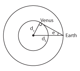
Notice how, in this planetary configuration, the Sun, Venus, and Earth form a right triangle with Venus situated at the right angle. The hypotenuse of the triangle, dE, is Earth’s orbital distance, i.e., the astronomical unit. The side of the triangle connecting Venus to the Sun, dV, is the size of the orbit of Venus, of course. So, using some trigonometry, we see that the ratio of Venus’s orbital radius to the astronomical unit is the sine of the angle (e) that Venus makes with the Sun:
Since we can easily measure the elongation angle by observing Venus as it moves through the sky during the year (it’s about 42 degrees), we can determine the size of Venus’s orbit in AU. But this is only part of the task. What we want is the size of the AU in meters or some other known unit. To get that, we must view Venus when it is crossing the Sun.
Because Venus’s orbit lies between Earth and the Sun, the planet periodically crosses in front of the disk of the Sun as seen from Earth. Such transits, as they are called, do not happen as often as we might think. This is because Venus and Earth orbit in slightly different planes. The orbital plane of Venus is tilted by a bit more than 3 degrees with respect to the ecliptic, the name given to Earth’s orbital plane. The Sun, however, is only about half a degree in diameter. That means that Venus must pass between Earth and the Sun while it is within a quarter degree of the ecliptic. This alignment is actually quite rare. Transits come in pairs separated by 8 years, but successive pairs are separated by about 120 years. Usually, Venus passes above or below the Sun, and no transit is visible.
However, occasionally, Venus does pass directly in front of the Sun. When that happens, two observers on Earth, at points A and B in Figure B.6.2 for example, might view the event as shown. Notice that they observe a small angular shift (exaggerated greatly in the figure) of Venus against the Sun’s surface. This shift is the key to determining the size of the astronomical unit.

In the triangle made between Earth and Venus, the short side, AB, can be measured if the latitude and longitude of each site are known. The angle can be determined by comparing the two observations. Then, using the small-angle approximation, we can deduce the long sides of the triangle. This is the difference in size of the orbit of Venus and Earth’s orbit.
But, we have already determined the ratio of these two distances, so we have two equations with two unknowns, and we can solve for either or both unknown. Using the ratio to eliminate dV, we get:
This is how the astronomical unit was originally determined. The method was first employed, without great success, because of the small separation between observing points, in 1639. More successful measurements, the result of large international expeditions, were done in 1761 and 1769, and again in 1874 and 1882. The last two transits of Venus were on June 8, 2004 and June 6, 2012. There will not be another transit of Venus until December 2117, and then 8 years later in 2125.
Much more precise determination of the astronomical unit is now possible by bouncing radio signals off of Venus and using time of flight to measure its distance.
There are no star clusters that are close enough to the Sun to have their distances determined through ground-based parallax measurements. Fortunately, it turns out that for one nearby star cluster, the Hyades, parallax is not the only means to measure distance. By using an alternative method to get an accurate distance to this cluster, we can use it to determine the distances to all other star clusters. Below, we explain how this is done.
We generally imagine that the stars are fixed in the sky, but that is not true. The stars appear to be fixed because of their great distances and the relatively short times (our lifetimes) we have to look at them. It would take millions of years for us to notice with our eyes alone that the relative position of stars had changed. With telescopes, these motions can be measured in just a few years or decades. The motion of the stars in the Hyades is what allows us to measure their distance. The technique used is called the moving cluster method.
To understand how this technique works, imagine you are watching the stars in the Hyades move over a very long period. If the cluster is moving away from you (which it is), then it will appear to get smaller and smaller over time. If you could watch it long enough, it would finally vanish into some point in the sky called the convergence point. This is not different from what happens if we watch a car drive away from us on a long, straight highway where our view is unobstructed. Eventually, the car disappears into a point near the horizon. The two sides of the road also seem to meet at this point.
Of course, if the star cluster is moving toward us, then we will see it emerge from the convergence point and grow larger with time (just as a car would if it traveled toward us). This effect is that of perspective, known to all students of drawing and painting.
Animated Figure 6.7: In this animation, the car vanishes into the convergence point as it drives away from the observer. Credit: NASA/SSU/Dominic Nicholson
To understand how the moving cluster method can be used to measure the distance to the Hyades, we have to break down the stellar motions into their components. All motion can be treated this way. In this case it is most convenient to view separately the motion of a star across our line of sight, and its motion along the line of sight. The former is called the star’s proper motion and is an angular measure. A star’s proper motion is related to its tangential velocity through space, vT, but is distinct from it. Proper motion is an angular motion, since all we can do is measure the change in the direction to the star over time. We cannot tell if this change in direction is due to the star being nearby and having a relatively small tangential velocity, or if the star is far away, but possesses a larger tangential velocity. Consider how the small-angle approximation applies here, and you will understand why this is so.
The proper motion will tell us where the convergence point lies. Assuming that the random motions of the stars within the cluster are small, proper motions of all the cluster stars will point to the convergence point.
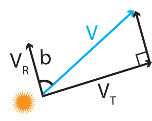
The other component of motion we can measure is called the star’s radial velocity, \(V_R\), which is its speed along our line of sight. For that we use the Doppler shift of the star’s spectral lines to determine its speed according to the Doppler formula.
Here, \(\Delta\lambda\) is the shift in the wavelength of some spectral line, \(\lambda\) is the rest wavelength of that line, and \(c\) is the speed of light. Of course, the actual velocity of the star through space is a combination of its radial velocity and its tangential velocity. Figure 6.9 shows the relationship between proper motion, radial velocity, and actual velocity. Notice that the radial velocity and tangential velocity form the perpendicular sides of a right triangle, and the total velocity forms the hypotenuse of this triangle. Once we know one of the sides and one of the angles in a right triangle, we can find all the unknown sides using trigonometry. And just a reminder: the radial velocity, \(V_R\), points toward or away from Earth, depending on whether the cluster moves toward us or away from us.
Now we use some geometry, and the fact that parallel lines meet at a point infinitely far away, to deduce one of the angles in the right triangle made up of the stellar velocity components. This geometry is depicted in Figure 6.10.
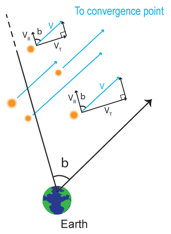
From Figure 6.10, we see that the angle, b, between any star and the convergence point will be the same as the angle between its radial velocity and its total velocity. This is because the convergence point is located infinitely far away, and from Euclidean geometry, parallel lines will meet at infinity. We can now use this and a little trigonometry to calculate the star’s tangential velocity from its radial velocity and the angle \(b\).
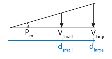
This velocity (\(V_T\)) relates to the proper motion as in Figure 6.8. We can use the small-angle approximation for the geometry of Figure 6.8 to write the distance as follows.
And solving for \(d\), we have the following.
So, to recap, if we are able to measure the proper motion for the stars in a cluster, we can determine where the cluster’s convergence point lies. Knowing the proper motion, the radial velocity, the convergence point, and the angular distance from the cluster to the convergence point gives us another geometrical distance determination method.
This method was the one used to determine the distance to the Hyades before the advent of space-based parallax measurements. An interesting aspect to this is that only the Hyades cluster is close enough for this method to work well. All other star clusters are too distant. As a result, all measurements to objects farther away than the Hyades were once dependent upon an accurate distance to that cluster. Astronomers understandably expended a large effort to get as accurate a measurement of the Hyades distance as possible. Since Hyades distance measurements were only accurate to about 15% from the ground, it meant that nearly all distances had this same uncertainty attached to them. Only the stars close enough for accurate parallax measurements had more precise distance measurements. With the advent of space-based parallax measurements, these distance uncertainties have greatly decreased. The Hipparcos satellite’s distance to the center of the Hyades is 46.34 ± 0.27 pc, a precision of only about half a percent.
This page titled 6.1: Geometrical Methods is shared under a CC BY-NC-SA 4.0 license and was authored, remixed, and/or curated by Kim Coble, Kevin McLin, & Lynn Cominsky.